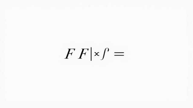
In the field of financial analysis and econometrics, the joint F statistic plays a significant role in evaluating the effectiveness of multiple independent variables in a regression model. It is especially relevant in the CFA curriculum when studying multiple linear regression and hypothesis testing. The joint F statistic formula helps determine whether a group of variables together explains a significant portion of the variation in the dependent variable. Understanding this concept and how to apply the formula is critical for finance professionals and students preparing for the CFA exams.
Understanding the Joint F Statistic
The joint F statistic is used in multiple regression analysis to test the null hypothesis that all slope coefficients (except the intercept) are equal to zero. In simple terms, it answers the question: Do the independent variables in this model, taken together, significantly explain the variation in the dependent variable?
This is different from testing individual coefficients, which is done using t-tests. The F-test assesses the overall significance of the regression model by comparing it to a baseline model that contains only the intercept.
Formula for the Joint F Statistic
The most commonly used formula for calculating the joint F statistic in the CFA context is as follows:
F = [(RSSr- RSSur) / q] / (RSSur/ (n - k - 1))
Where:
- RSSr= Residual Sum of Squares for the restricted model (model without certain independent variables)
- RSSur= Residual Sum of Squares for the unrestricted model (model with all independent variables)
- q= Number of restrictions or number of variables being tested jointly
- n= Total number of observations
- k= Number of independent variables in the unrestricted model
Alternatively, when using R-squared values, another form of the joint F statistic formula is:
F = [(R² / k)] / [(1 - R²) / (n - k - 1)]
This version is applicable when you are testing the entire model (i.e., whether all slope coefficients equal zero). It is commonly used in practice because R-squared is readily available in regression output.
Interpreting the Joint F Statistic
The result of the F-test is compared to a critical value from the F-distribution withqand(n - k - 1)degrees of freedom. If the F-value is greater than the critical value, the null hypothesis is rejected, indicating that the model has significant explanatory power.
Steps in Interpretation
- Calculate or obtain the F statistic from regression output.
- Determine the critical F value at the desired significance level (e.g., 5%).
- If F > Fcritical, reject the null hypothesis.
- This means that the independent variables, taken as a group, significantly explain the variation in the dependent variable.
Application in CFA Exam Context
In the CFA curriculum, especially in Level II, the joint F test is covered in the context of multiple linear regression. Candidates are expected to understand when and how to use it, and how to interpret the results. Questions may involve evaluating regression outputs, calculating the F statistic using provided data, or interpreting whether the model is statistically significant.
Example Scenario
Suppose a regression model is created to predict stock returns based on three economic indicators: interest rates, inflation, and GDP growth. An analyst wants to test whether these three indicators together explain a significant portion of the variance in stock returns.
Using the unrestricted model (which includes all three variables), and comparing it to a restricted model (intercept only), the joint F statistic can be calculated. If the F-test shows a high value that exceeds the critical threshold, the analyst can conclude that the economic indicators jointly have explanatory power.
Assumptions Behind the Joint F Test
For the joint F statistic to be valid, several assumptions underlying multiple linear regression must be met:
- Linearity: The relationship between independent and dependent variables should be linear.
- No multicollinearity: Independent variables should not be highly correlated with each other.
- Homoscedasticity: The variance of the error terms should be constant across observations.
- Normality of errors: The error terms should be normally distributed for small sample inference.
- Independence: Observations should be independent of one another.
If these assumptions are violated, the results of the F test may not be reliable, and alternative techniques or model adjustments may be necessary.
Limitations of the F Statistic
While the joint F test is useful, it also has its limitations:
- It does not tell which variables are significant: The F-test only tells you whether the group of variables is significant as a whole, not which specific ones are driving the result.
- It is sensitive to sample size: With a large sample, even small differences can appear statistically significant.
- Overfitting risk: Adding more variables may increase R-squared, leading to a higher F-value, even if those variables are not meaningful predictors.
Therefore, the F test should always be used in conjunction with other tools such as adjusted R-squared, t-tests for individual coefficients, and theoretical justification for including variables in a model.
The joint F statistic is a fundamental concept in multiple regression analysis and a core part of the CFA curriculum. It provides a way to evaluate whether a group of independent variables, taken together, has a statistically significant relationship with the dependent variable. By understanding the formula, interpreting the results correctly, and recognizing the assumptions and limitations, analysts and CFA candidates can better assess the strength and relevance of regression models in real-world financial analysis.
